
 |
Protein Crystallography Course
|
The basic idea of maximum likelihood is quite simple: the best model is most consistent with the observations. Consistency is measured statistically, by the probability that the observations should have been made. If the model is changed to make the observations more probable, the likelihood goes up, indicating that the model is better. (You could also say that the model agrees better with the data, but bringing in the idea of probability defines "agreement" more precisely.)
The probabilities have to include the effects of all sources of error, including not just measurement errors but also errors in the model itself. But as the model gets better, its errors clearly get smaller, which means the probabilities become sharper. The sharpening of probabilities also increases the likelihood, as long as they are no sharper than appropriate. This will be clear in the illustrative example below.
Mathematically, the likelihood is defined as the probability of making the set of measurements. If you have N observations of different quantities xj, for instance, then the likelihood is defined as:
![]()

The assumption of independent probabilities certainly makes life simpler, because joint distributions can be extremely difficult to work with! But you may lose something if the errors are correlated, so it is important to be careful.
Sums are easier to deal with than products (and the product of a lot of small numbers may be too small to represent on a computer), so we generally work with the log of the likelihood. The log varies monotonically with its argument (i.e. ln(x) increases when x does and decreases when it does), so the log of a function will have its maximum at the same position. Usually what we are interested in is finding the position of the maximum of the likelihood function.

In fact, to make the analogy with least-squares (see below) more obvious, we often minimise minus log likelihood.
Though the basic ideas behind maximum likelihood are quite simple, the difficult part is working out the probability of making an observation. For crystallographic refinement (the case we will consider later in this lecture), we have worked out much of the background in the previous lecture.
One way to think about likelihood is that we imagine we haven't measured the data yet. We have a model, with various parameters to adjust (coordinates and B-factors in the case of crystallography), and some idea of sources of error and how they would propagate. This allows us to calculate the probability of any possible set of measurements. Finally, we bring in the actual measurements and see how well they agree with the model.
The behaviour of a likelihood function will probably be easier to understand with an explicit example. To generate the data for this example, I generated a series of twenty numbers from a Gaussian probability distribution, with a mean of 5 and a standard deviation of 1. We can use these data to deduce the maximum likelihood estimates of the mean and standard deviation.
First we need a probability distribution to define the likelihood function. Now, as discussed in the last lecture, the central limit theorem means that a Gaussian distribution is often an appropriate choice. Since I generated the data from a Gaussian distribution, this is obviously such a case!
The likelihood function, then, will be the probability of generating our twenty data points. The parameters of this likelihood function are the mean and standard deviation we assume for the Gaussian probability distribution. It is important to realise that, in maximum likelihood, the standard deviations can also be full-fledged parameters. (If we have good estimates of the standard deviations of measurement errors, based either on theory or on replicate measurements, of course we use those error estimates instead of refining them.)
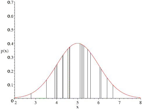
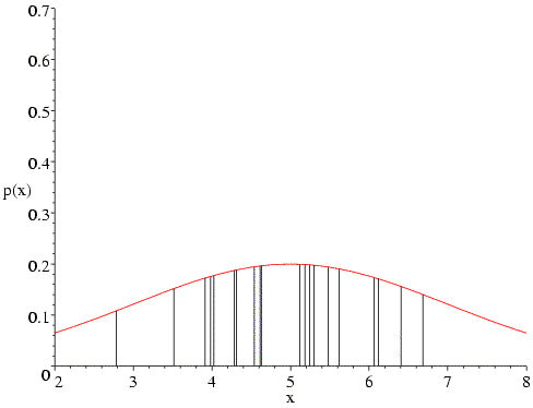
In the following figure, the Gaussian probability distribution is plotted for a mean of 5 and standard deviation of 1. The twenty vertical bars correspond to the twenty data points; the height of each bar represents the probability of that measurement, given the assumed mean and standard deviation. The likelihood function is the product of all those probabilities (heights). As you can see, none of the probabilities is particularly low, and they are highest in the centre of the distribution, which is most heavily populated by the data.
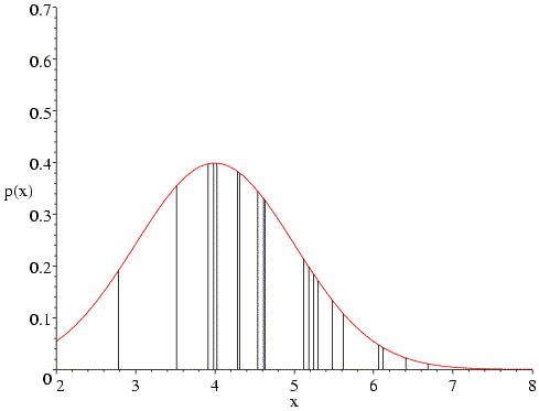
What happens if we change the assumed mean of the distribution? The following figure shows that, if we change the mean to 4, the data points on the high end of the distribution become very improbable, which will reduce the likelihood function significantly. Also, fewer of the data points are now in the peak region.
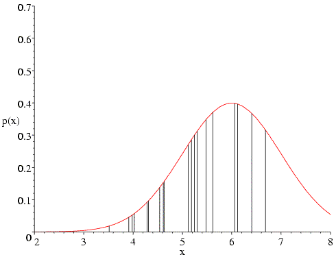
The same sort of thing happens if we change the mean to 6.
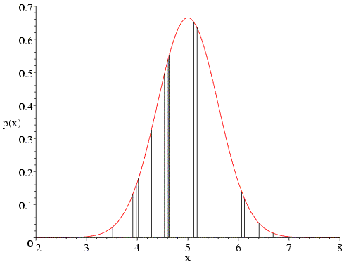
What happens if we have the correct mean but the wrong standard deviation? In the following figure, a value of 0.6 is used for the standard deviation. In the heavily populated centre, the probability values go up, but the values in the two tails go down even more, so that the overall value of the likelihood is reduced.
Similarly, if we choose too high a value for the standard deviation (two in the following figure), the probabilities in the tails go up, but the decrease in the heavily-populated centre means that the overall likelihood goes down. In fact, if we have the correct mean the likelihood function will generally balance out the influence of the sparsely-populated tails and the heavily-populated centre to give us the correct standard deviation.
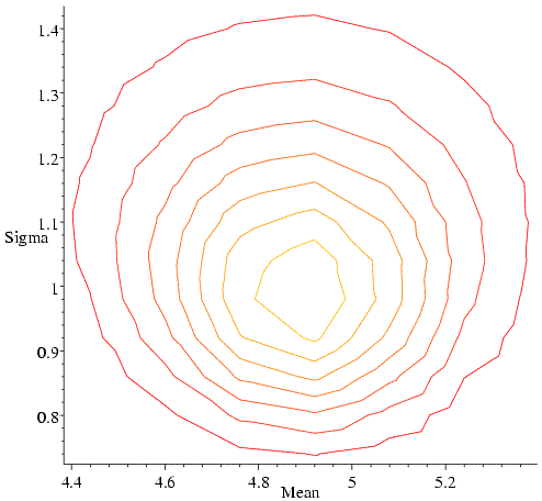
In fact, we wouldn't generally choose to maximise such a likelihood function by systematic search, because it turns out that we could have solved the likelihood equations analytically. If we did this, we would have obtained the classical least-squares answer (estimate of the mean is the mean of the data, estimated variance is the sum of the squared deviations from the mean). As an aside, you may remember that such an estimate of the variance (standard deviation squared) is an underestimate, because it doesn't take account of the degrees of freedom in fitting the equation. So the maximum likelihood estimate is not what a statistician would call an unbiased estimate. We should keep this in mind when we think about overfitting in structure refinement, but we won't be worrying about it in detail.
Many people working on optimisation problems believe that maximum likelihood provides the best framework. Nonetheless, least-squares methods are almost ubiquitous. People who favour likelihood would say that this is only because Gaussian distributions arise so often in the underlying probabilities. The problem is that least-squares methods are often used even when they are not appropriate. It turns out that this is the case for many applications in crystallography. As we will see, the reason for this is (indirectly) the phase problem. Many sources of error in crystallography have their effect in the complex plane, for instance model errors or lack of isomorphism, but we only measure amplitudes or intensities.
Let's apply maximum likelihood to a problem where the errors in predicting the observations follow a Gaussian distribution. We will see, with a few simple manipulations, that maximum likelihood is equivalent to least squares in this case.
First, remember the equation for a Gaussian probability distribution.

In log likelihood, we will need the log of this probability distribution

Now, the likelihood is the probability of making the entire set of observations. As before, we are assuming that the observations are independent, so that the likelihood is the product of all the individual probabilities and the log likelihood is the sum of the logs. To make the comparison with least-squares minimisation clearer, let's stick a minus sign in front and show the equation for minus log likelihood.

Compare this to the weighted sum of squares residual used in least-squares minimisation.

The log of 2π will not change in -LL. If we assume that the standard deviations (measurement errors) are also constant, then -LL differs from WSSQ only by a factor of two and will obviously find the same optimal solution.
In structure refinement, we will find that:
so that the use of least squares is not really justified.
Until a few years ago, it was assumed that crystal structures should be refined by minimising the sum of squares of deviations between the observed and calculated amplitudes or intensities. But in the last few years, maximum likelihood methods have been introduced and have quickly caught on because they are more successful.
You might think that Gaussian distributions are so ubiquitous that least-squares would be the correct choice. After all, we saw in the last lecture that various important structure factor distributions are indeed Gaussian in form. But the errors in these structure factor distributions are Gaussian in the complex plane, whereas we measure intensities (which can be converted into amplitudes). To use the structure factor distributions to predict amplitudes, we have to average over all possible values of the phase, and this changes the nature of the error distributions.
Before the advent of maximum likelihood, there were hints of problems with least-squares minimisation. For instance, in least squares the squared deviations should be weighted by the inverse of the variance of the observation, as shown in the equation below. But refinements weighted by the actual measurement errors did not converge well. It was found by trial and error that the best results were obtained if the weights were based on standard deviations proportional to the rms difference between |FO| and |FC| in the current model.

As well, it was found by trial and error that it was sometimes best to completely eliminate data at high resolution until the model had improved. One would expect that a proper treatment of errors would effectively ignore data that do not contribute constructively to refinement. This is what turns out to happen automatically with maximum likelihood.
The least-squares target looks like it is independent of the phases, but in fact it implicitly assumes that the phases are essentially correct. We can see this by using Parseval's theorem to see what is the real-space equivalent of the least-squares target. Remember that Parseval's theorem says that the rms error on one side of the Fourier transform is proportional to the rms error on the other side of the Fourier transform. The rms error in the structure factors involves a vector difference, but we can turn our amplitude difference into a vector difference by assigning both amplitudes the calculated phase.

Ignoring the weighting term, minimising the least-squares target turns out to be equivalent to minimising the rms difference between the electron density of the model (Fourier transform of FC) and a map computed with the observed amplitudes and calculated phases. You can see why refinement against such a target might converge poorly, because the map computed with observed amplitudes and calculated phases is biased to resemble the model.
In fact, we really can't get away from phases. This can be seen in another way by considering what the diffraction data can tell us about possible atomic positions.
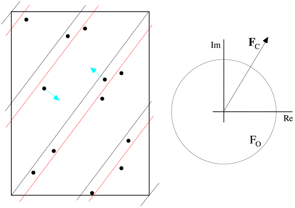
Ignoring for the moment any experimental phase information that we might possess, each diffraction amplitude tells us something about the distribution of the atoms relative to one set of Bragg planes. If the amplitude is weak, then the atoms are scattered randomly with respect to that set of planes and their contributions to the structure factor tend to cancel out. If the amplitude is strong, then the atoms tend to be concentrated in planes parallel to the Bragg planes.
This is illustrated below. In the figure on the left, the dots represent atoms, and the black lines indicate the Bragg planes, one of which passes through the origin so that atoms on the planes would scatter with a phase of zero. The red lines indicate the planes corresponding to the phase of the structure factor computed from the model; these are the planes with the Bragg spacing around which the atoms tend to concentrate. In the figure on the right, the calculated structure factor is indicated as the vector FC, while the observed amplitude is indicated with a circle of radius |FO|. The calculated amplitude is larger than the observed amplitude, indicating that the atoms are concentrated too much about planes parallel to the Bragg planes. To make the model agree better with the data, then, the atoms can be moved away from the red planes, as indicated with blue arrows for two atoms. This is how refinement uses the observed diffraction data. Of course, every reflection gives information about a different set of planes, and they're all taken into account when the atoms are shifted.
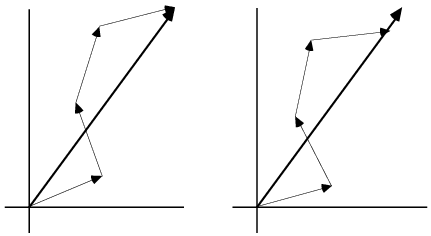
The effect of shifting the atoms away from the planes defined by the current phase is to rotate their contribution to the overall structure factor away from the total structure factor. In the figure below, you can see how this leads to a reduction in the calculated amplitude (and also how it tends to preserve the current phase!). The amplitude can also be changed by changing the B-factors of individual atoms: if the B-factor of an atom contributing in the direction of the overall structure factor is increased, the overall amplitude will be decreased. The amplitude can also be decreased by decreasing the B-factor of an atom contributing in the opposite direction to the overall structure factor.
Unfortunately, there is a bit of a complication. If we improve agreement in this way we are implicitly assuming that the phases are correct. If |FC| is too large, the atoms are too concentrated about some set of planes parallel to the Bragg planes, but not necessarily the ones corresponding to the current calculated phase. So perhaps all the atoms on the lower right of the red planes should be moved further to the lower right, reducing the amplitude and simultaneously changing the phase. Or maybe all the atoms on the upper left should be moved further to the upper left. The problem is that we don't really know. Another way to look at this is that, when we decide how to move one atom, the decision depends on the position of all the other atoms, and if they're not in the right place, then we won't necessarily move that atom in the right direction. This is why crystallographic refinement is iterative; as the model gets better, the shifts become more accurate.
Notice, as well, that if an atom is more than 1/2 of the d-spacing away from its correct position, shifting it in the wrong direction may be the easiest way to improve the amplitude agreement. This is why we should downweight the higher resolution data until the agreement starts to improve. (This happens automatically with maximum likelihood.)
So refinement is not just a matter of making the calculated amplitudes equal to the observed ones. It turns out that, to make the best decision about how to move an atom, we need to have an idea of the overall accuracy of the model, which affects the accuracy of the phases.
Since we can't escape from the phases, we had better account for the ambiguity in their values. It turns out that maximum likelihood provides a natural way to do this.
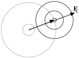
As we have mentioned, the structure factor probability distributions derived in the last lecture are Gaussians in the complex plane. But we measure intensities or amplitudes, so if we want to predict the observations from our model, we have to convert the structure factor probabilities into a form that applies to amplitudes. The structure factors can be considered either as complex numbers with real and imaginary parts, or as having an amplitude and phase. To get a distribution expressed in terms of amplitudes, we have to convert first to the amplitude/phase description and then integrate out the phase. (In general, extra random variables in a joint probability distribution can be eliminated by integration.) This integration is shown schematically in the following figure.
 |
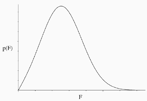 |

In statistical theory, the result of this integration is called a Rice distribution, but the same distribution has been used in crystallography by Luzzati and Sim and their successors. We won't bother for now with its mathematical form, which can be found in the original literature.
The Rice distribution accounts for the effect of model error on our ability to predict the observed amplitude, but we have not yet accounted for the effect of observation error. Three methods are used in practice:
In practice, the three methods are similar, although MLI seems to give slightly better results than MLF.
The following figure shows that the likelihood function can be a bit counterintuitive, but it is important to realise what is going on. The top part shows the 2D Gaussian distributions corresponding to a weak FC (left), a moderate one (centre) and a strong one (right). Even from these pictures, you can see that when FC is unusally small or large, the true structure factor will probably be closer to average in amplitude.
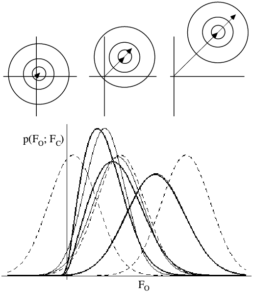
The lower part of the figure shows probability distributions corresponding to the top three cases. For each case, the Rice distribution is shown (thick lines), along with the MLF approximation (thin lines) and a Gaussian centred on |FC|. If we were using a least-squares target, we would be assuming these Gaussian distributions were correct. And even though it seems intuitively reasonable that FC should only be small when |FO| is, a proper analysis of the effect of model errors tells us that this isn't necessarily so.
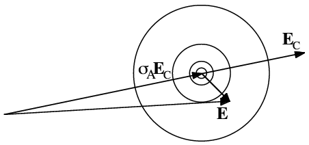
In the last lecture, we saw that the structure factor probability distributions depend on a single parameter, σA. Both the centre of the 2D Gaussian distribution and its width are affected by σA, so the quality of the maximum likelihood refinement depends very sensitively on the quality of the estimate of σA. As the following figure illustrates, σA is essentially the fraction of the normalised structure factor that is correct. As σA decreases, the fraction that is correct decreases and the size of the Gaussian error increases. It should be noted that σA is a function of resolution, because model errors have a bigger effect on structure factor agreement at high resolution than at low resolution.
In the program SIGMAA, the parameter σA is estimated as a function of resolution by maximising the same Rice likelihood function that is used in structure refinement. At a particular resolution, the correct value of σA will give the best prediction of the distribution of observed amplitudes from the calculated amplitudes. This is analogous to the example given above, where the correct standard deviation for a Gaussian distribution maximised the likelihood.
The importance of a good estimate for σA is highlighted by the following figure. Three probability curves are shown, corresponding to different assumed values of σA. The red vertical line indicates that a particular value of the observed amplitude may be very improbable or highly probable, depending on the estimate of σA.
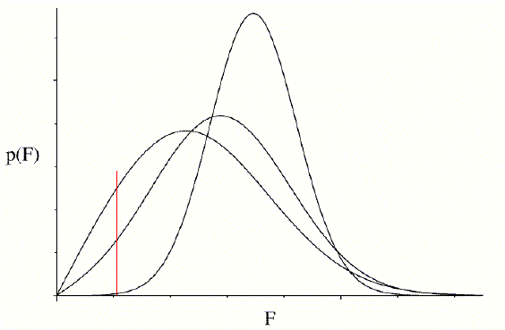
Since maximum likelihood refinement is based directly on these probabilities, the course of refinement depends very sensitively on having good estimates. Also, as refinement progresses, the model should improve and σA values should increase, so it is important to update the estimates at intervals. In principle, as mentioned earlier, unknown variance parameters are refineable parameters in maximum likelihood. Unfortunately, if we try to refine σA values at the same time and with the same data as the atomic parameters, we get into trouble. In a typical protein structure refinement, there are too many parameters for the number of observations and the data are severely overfit. (Typical observation to parameter ratios can be seen in notes from an earlier lecture.) The σA values are then overestimated and the quality of the likelihood target suffers severely. Currently, the best way around this problem is to estimate σA separately with the cross-validation data that are used to compute Rfree.
Occasionally there are arguments about whether cross-validation should be used throughout refinement, or just to validate a particular refinement strategy. With maximum likelihood refinement, these arguments are irrelevant at the moment. The refinement targets depend sensitively on the estimates of σA, and the only way to get these estimates at the moment is to use cross-validation.
We won't get into the details here, but it turns out that the standard algorithm in SIGMAA is impractical for use with cross-validation data. The standard algorithm divides reciprocal space into shells containing 500-1000 reflections, and a value for σA is estimated independently for each shell. That number of reflections is needed to reduce the statistical error in the σA estimates to an acceptable level. Unless you're working on the structure of a virus or the ribosome, you won't be able to set aside that many cross-validation data!
Instead, what is done is to exploit the fact that σA varies smoothly with resolution. By simply adding a restraint that every σA value must lie close to the line joining its neighbours, the total number of cross-validation data required is reduced to about 1000. If you have a large unit cell and can afford to, it's worth setting aside up to about 2000 reflections. On the other hand, if you have fewer than 10,000 reflections in total, it's best to use no more than 10% of the data for cross-validation and accept that the σA estimates won't be quite as accurate.
A special case arises when there is very high non-crystallographic symmetry (NCS). As we will see in the upcoming lecture on density modification methods, the existence of NCS implies statistical relationships between structure factors. With high NCS, there is a very real danger that the cross-validation data are no longer independent of the working data. So overfitting of the working data can propagate into the cross-validation data. The statistical relationships connect structure factors related by the NCS rotation operations, so correlated structure factors will all have the same (or similar) resolution. So the danger of overfitting propagating into the cross-validation data can be reduced by selecting the cross-validation data in thin resolution shells. This seems to work in practice, although a systematic test has not been carried out.
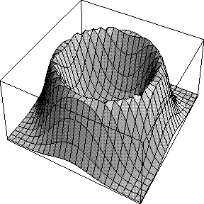
When we integrated around the phase circle to turn the 2D Gaussian structure factor probability distribution into a Rice distribution, we implicitly assumed we had no phase information other than the calculated structure factor, i.e. that all possible phase values were equally probable. The effect is that the likelihood target depends only on the amplitude of FC and not on its phase. This is illustrated in the figure below, which indicates the likelihood contributed by a single reflection as a function of FC: the real part of FC runs along the horizontal axis and the imaginary part along the vertical axis.
On the other hand, if we do have prior phase information, we can use this to weight the integral. The prior phase information can be expressed in terms of Hendrickson-Lattman coefficients, as mentioned in the last lecture.
![]()
The integral over the phase is then carried out as shown in the following equation:

Now the likelihood does depend on the phase of FC. In the figure below, a phase probability curve is shown on the left, and on the right is the likelihood as a function of FC, with its real and imaginary parts. When the calculated phase reinforces one of the phase choices from the prior phase distribution, the likelihood score is much higher.
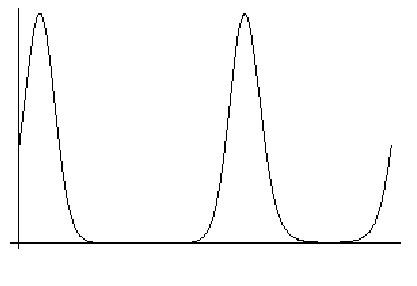
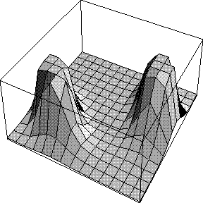
The likelihood target using prior phase information is called MLHL (Maximum Likelihood using Hendrickson-Lattman coefficients) and is available in X-PLOR, CNS and Refmac. It is much more powerful than the unphased targets and should be used whenever phase information is available.
As noted above, a big problem with macromolecular structure determination is the poor observation:parameter ratio at the resolutions to which crystals normally diffract. If we simply refine the positions and B-factors of all the atoms, the refinement will be poorly behaved, the data will be terribly overfit, and the resulting atomic model will probably be very poor.
The way we deal with this is either to add "observations" in the form of restraints, or reduce the number of parameters by constraining the model in some way. Typical restraints include bond lengths, bond angles and van der Waals contact distances. There are generally also restraints to keep planar groups planar, and to maintain the chirality of chiral centres. The restraints are entered as terms in the refinement target, and are weighted so that the deviations from ideal values match the deviations found in databases of high resolution structures.
Constraints are a bit different. When you constrain a structure, you are actually changing the parameterisation to reduce the total number of parameters. One possibility is to allow only torsion angles to be adjusted, instead of all the individual x,y,z coordinates. Another very common case occurs when there are multiple copies of a molecule in the asymmetric unit of the crystal. The model can be a single copy of the molecule, replicated by rotations and translations to create the other copies. So if, for instance, there are three copies in the asymmetric unit, the number of adjustable parameters can be reduced by a factor of three.
It turns out that there is a way of looking at likelihood that brings restraints in naturally, by interpreting the restraints as bringing in the a priori probability of different possible models. To understand this requires us to digress a bit into more likelihood theory.
The principle of maximum likelihood is quite intuitive, and it leads to useful results, but you might argue that there is a logical problem. The likelihood function is the probability of the data given the model (p(data;model), in more formal notation), but we tend to think of it as the probability that the model is a good reflection of reality, given the data (p(model;data)). The two are not equivalent. The two probabilities are related by Bayes' Theorem, and the application of Bayes' Theorem can give us new insight into likelihood. (It should be noted that this issue is a bit contentious, and some statisticians feel that it is not necessary to invoke Bayesian reasoning.)
Bayes' Theorem concerns the relationship between conditional probabilities. For instance, p(A;B) is the probability that A is true, given that we know that B is true. If A depends on B, then this will be different from p(A), which is the overall probability that A is true, regardless of whether or not B is true.
Bayes' Theorem is easily derived starting from the multiplication law for probabilities.
p(A,B) = p(A)p(B;A)
This can be illustrated with a Venn diagram.
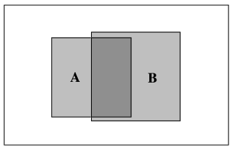
In the Venn diagram, the whole box represents all possibilities. The box labelled A represents the probability that A is true. Since A occupies 20% of the whole box in this diagram,
p(A) = 0.2
The box labelled B represents the probability that B is true, and
p(B) = 0.25
The region of overlap represents the probability that both A and B are true.
p(A,B) = 0.1
If we assume that A is true, half of the time B will also be true.
p(B;A) = 0.5 = 0.1/0.2 = p(A,B)/p(A)
If we assume that B is true, 40% of the time A will also be true
p(A;B) = 0.4 = 0.1/0.25 = p(A,B)/p(B)
Now we can verify the multiplication law for probabilities, with two different expressions derived from the last two equations.
p(A,B) = p(A) p(B;A) = 0.2*0.5 = 0.1
= p(B) p(A;B) = 0.25*0.4 = 0.1
Bayes' theorem is then derived simply as follows:
p(A,B) = p(A) p(B;A) = p(B) p(A;B)

Translating this into likelihood terminology, we have:

The data are fixed and we are only varying the parameters of the model, so the denominator is just a normalisation constant. If we want to maximise likelihood, the value of a constant factor won't change the position of the maximum, so:
L(model;data) = p(model) p(data;model)
If we have no reason to prefer one model over another, in the absence of data, we are back to the original expression for likelihood. However, if we do, then we should include the a priori probability of the model in the likelihood function, which can then be thought of as the product of the model likelihood and the data likelihood. If we take the log, we use the sum of the log likelihood of the model and the log likelihood of the data given the model.
In structure refinement, restraints to ideal geometry can be thought of as expressing the a priori probability of the model. In this analysis, any prior information about the probability of certain features in real proteins could legitimately be introduced. In any event, we need restraints to get around the problems of the typical parameter to observation ratio in protein structure refinement, which was mentioned above.
Restraints supply information about the allowed geometry of the molecules we are dealing with: bond lengths, bond angles, van der Waals contacts, even preferred torsion angles. In terms of likelihood theory and the Bayesian interpretation, restraints should have a basis in probabilities. For instance, a bond length could be given a Gaussian probability distribution from small molecule observations. This will enter the log likelihood target as a weighted squared deviation:

where b is a particular bond length and σb is its standard deviation in database structures. The factor of two in the denominator keeps the term on the same scale as the data likelihood.
Another way to treat restraints is to include the calculated energy of the molecule (appropriately weighted) as part of the function being minimised. This can be interpreted as log likelihood information by considering the energies to represent Boltzmann probabilities.

The log likelihood term corresponding to this probability varies as ΔG/kT. So the energy term should be divided by kT to put it on the same scale as the data likelihood.
Note that, in principle, there is no question about the correct relative weights to use between the restraint terms and the data likelihood function. In practice, probably because of overfitting of the X-ray data, it is necessary to overweight the X-ray (data likelihood) terms to get the refinement to converge. As the resolution gets higher, the optimal weights come down towards the theoretical values, which makes sense because there is less overfitting with higher resolution data.
Pannu, N.S. and Read, R.J. "Improved structure refinement through maximum likelihood", Acta Cryst. A52: 659-668 (1996).
Murshudov, G.N., Vagin, A.A. and Dodson, E.J. "Refinement of macromolecular structures by the maximum-likelihood method", Acta Cryst. D53: 240-255 (1997).
Bricogne, G. and Irwin, J. "Maximum-likelihood structure refinement: theory and implementation within BUSTER + TNT" in Macromolecular Refinement: Proceedings of the CCP4 Study Weekend January 1996, Dodson, E., Moore, M., Ralph, A. and Bailey, S. (eds.), CCLRC Daresbury Laboratory, pp. 85-92 (1996).
Pannu, N.S., Murshudov, G.N., Dodson, E.J. and Read, R.J. "Incorporation of prior phase information strengthens maximum-likelihood structure refinement", Acta Cryst. D54: 1285-1294 (1998).
Notes from refinement workshop held in York, September 1997. These notes have been maintained by Jim Naismith.
© 1999-2009 Randy J Read, University of Cambridge. All rights reserved.
Last updated: 6 April, 2009