
|
Protein Crystallography Course |
This series will cover the theory and practice of X-ray crystallography, particularly as it applies to studying the three-dimensional structure of macromolecules. The notes will often refer specifically to proteins, but generally the same techniques and problems apply to other macromolecules (DNA, RNA) or assemblies (viruses, ribosomes).
If you've gotten this far you probably have a good idea why we want to study the 3D structure of molecules. 3D structure allows us to understand biological processes at the most basic level: which molecules interact, how they interact, how enzymes catalyse reactions, how drugs act. In some cases, it can allow us to understand disease at an atomic level, such as the sickling of red blood cells. We can also exploit 3D structure in developing new drugs.
There are a number of methods for studying 3D structure, outlined briefly in the next section. But we will concentrate on X-ray crystallography, which is arguably the most effective of these techniques at present. Certainly the other techniques complement crystallography and have a valued place in the set of tools that we use.
If you think about how you determine the shape of objects around you, the most obvious is just to look at them. If they're small, you use a microscope. But there's a limit to how small an object can be seen under a light microscope. The limit (the "diffraction limit") is that you can not image things that are much smaller than the wavelength of the light you are using. The wavelength for visible light is measured in hundreds of nanometers, while atoms are separated by distances of the order of 0.1nm, or 1Å. Looking at the electromagnetic spectrum, X-rays get us in the right wavelength range.
But we can't build an X-ray microscope to look at molecules, for two reasons. First, we don't have an X-ray lens. Second, even if we did have one, it would have to be made with tolerances significantly less than the distance between two atoms! However, we can (in effect) simulate an X-ray lens on a computer. You can think of a microscope as working in two stages. First, light strikes the object and is diffracted in various directions. The lens collects the diffracted rays and reassembles them to form an image. With X-rays, we can detect diffraction from molecules, but we have to use a computer to reassemble the image. It's not quite so simple, but that's the essence of the method.
We can consider other types of waves with wavelengths in the correct range. One of the wonderful and unexpected results of quantum mechanics is that particles have a wave nature. The faster they are moving, the shorter the wavelength. Two types of particles can be accelerated to speeds sufficient to bring their wavelengths into the Ångstrom range: neutrons and electrons. Neutron diffraction works more or less like X-ray diffraction.
Electrons diffract too, but they can also be focused by magnetic fields, which allows the construction of electron microscopes. The very best electron microscopes have resolving powers near atomic resolution. There are special problems with sample damage, which means that very low electron doses must be used to avoid destroying the sample, so that the images have extremely poor signal-to-noise and must be averaged. It turns out that electron microscopy tends to be most useful for very large assemblies, which is where crystallography tends to become very difficult, so that the techniques are quite complementary. But there won't be space or time to go into all of that here.
Apart from looking at things to determine their shape, you can also use your sense of touch. That, in essence, is what a number of techniques based on scanning microprobes do.
Here we stray from analogy with our senses. NMR uses much more indirect methods to determine 3D structure. It is based on the quantum mechanical properties of atoms, particularly spin, and it determines information about atoms from the fact that their local environment influences how they respond to applied magnetic fields. The kind of information that can be obtained includes the measurement of interatomic distances, and features of the spectrum (coupling constants) that can be interpreted in terms of torsion angles.
As noted above, the use of electromagnetic radiation to visualise objects requires the radiation to have a wavelength comparable to the smallest features that you wish to resolve. We often use X-rays emitted from copper targets bombarded with high energy electrons, which emit at several characteristic wavelengths: the one we use is called CuKα, which has a wavelength of 1.5418Å. This is very similar to the distance between bonded carbon atoms, so it is well suited to the study of molecular structure.
What we see as the result of a crystallographic experiment is not really a picture of the atoms, but a map of the distribution of electrons in the molecule, i.e. an electron density map. However, since the electrons are mostly tightly localised around the nuclei, the electron density map gives us a pretty good picture of the molecule.
This is because electromagnetic radiation (including X-rays) interacts with matter through its fluctuating electric field, which accelerates charged particles. You can think of the electrons fluctuating in position and, through their accelerations, emitting electromagnetic radiation in turn. Because electrons have a much higher charge to mass ratio than atomic nuclei or even protons, they are much more efficient in this process. Intensity of scattered radiation is proportional to the square of the charge/mass ratio, and the proton is about 2000 times as massive as the electron.
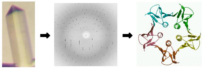
X-ray scattering from a single molecule would be incredibly weak and extremely difficult to detect above the noise level, which would include scattering from air and water. A crystal arranges huge numbers of molecules in the same orientation, so that scattered waves can add up in phase and raise the signal to a measurable level. In a sense, a crystal acts as an amplifier.
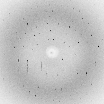
Of course, if the waves add up in phase in some directions, they have to cancel out in a lot of other directions. That is why the diffraction pattern from a crystal is an array of spots.
There are a number of potential bottlenecks in determining a crystal structure, but growing a useful crystal can be the most serious one. If you can't collect any data or only bad data, you won't be able to solve a structure. So we'll spend the next lecture looking at the theory and practice of crystallisation.
Think of the electrons in a crystal as emitters of little waves. When the little waves add up, they interfere with one another: they can add up in phase, out of phase, or something in between. Which of these they do depends on the direction of the incoming and outgoing waves and the positions of the electrons relative to each other. The total path from the source to the detector will determine what happens. If the difference in the lengths of the paths taken via one electron and another is a multiple of the wavelength, then the waves will scatter in phase and their amplitudes will add up. If it's a half-integral multiple of the pathlength, they will scatter exactly out of phase and cancel out.
The conditions for scattering in phase can be summed up quite neatly if you think of the waves being reflected off of planes passing through the atoms. The relationship between scattering angle and the interplanar spacing is given by Bragg's law, which we will go into analytically at a later date. For the meantime, there is a Bragg's law applet that allows you to play with wavelength, interplanar spacing and angle of incidence and reflection. Notice that, if you increase the wavelength, the total diffracted intensity becomes less sensitive to the spacing or to changes in angle. That means that the diffraction pattern becomes less sensitive to the fine details. Also notice that, if you keep the wavelength fixed but decrease the spacing, you have to go to higher angles to get the first peak in diffracted intensity. Because of this inverse relationship between the spacing in the object and the angle of diffraction, the diffraction space is usually called "reciprocal space". The further out you go in reciprocal space, the more the diffraction pattern becomes sensitive to objects that are close together in "real space". We'll spend a lot of time later dealing with the properties of reciprocal space and how to think about it.
One more thing to notice: the position of the peaks in the wave that results from the interference of scattering from two atoms depends on their relative position. The position of the peak in a wave is described by its phase.
It turns out (for reasons that we'll go into in great depth in the advanced series) that the diffraction pattern is related to the object diffracting the waves through a mathematical operation called the Fourier transform. If you think of the electron density as a mathematical function, then the diffraction pattern is the Fourier transform of that function.
This means that, for a real understanding of crystallography, you need to understand some properties of Fourier transforms, and we'll spend some time on that later. But for now we'll content ourselves with one property of Fourier transforms: they can be inverted. If you apply a Fourier transform to some function, you can take the result and run it through an inverse Fourier transform to get the original function back. (The inverse Fourier transform is essentially just another Fourier transform.) This is how we can use a computer to take the diffraction pattern and give us a picture of the electron density.
But there's a problem, and it's such an important problem that it's usually referred to in capital letters as The Phase Problem. The Phase Problem arises because we need to know both the amplitude and the phase of the diffracted waves to compute the inverse Fourier transform. But what we measure in the experiment is essentially a count of the number of X-ray photons in each spot. We have no practical way of measuring the relative phase angles for the different diffracted spots experimentally. The number of photons gives the intensity, which turns out to be proportional to the square of the amplitude (peak height) of the diffracted wave. But the phase has been lost.
The phase, in fact, is extremely important, as you can see from taking a look at Kevin Cowtan's Book of Fourier.
Kevin has another useful web page, the Interactive Structure Factor Tutorial, which provides a nice tool to get a feel for how the inverse Fourier transform works.
Apart from growing useful crystals, this is often the most serious bottleneck in determining a new structure. Because we can't measure the phase directly, we have to deduce it indirectly. We'll go into this in more detail later, but there are basically two approaches:
The classic technique along these lines is isomorphous replacement. Isomorphous means "same shape" and, essentially what you do is to get a crystal that is nearly identical to the one you're studying, except that a few atoms have been replaced or added. If these atoms are "heavy", i.e. they have a large atomic number, they will perturb the diffraction pattern. It is possible to deduce the positions of the few heavy atoms and from that to deduce possible values for the phase angles.
A conceptually similar technique uses just one crystal, which contains atoms called anomalous scatterers. By changing the wavelength of the X-rays, you can change the degree to which the anomalous scatterers perturb the diffraction pattern, which gives the same kind of information as isomorphous replacement. This technique, called multiple-wavelength anomalous dispersion (MAD) will be covered in its own lecture in the advanced series.
If you have a good idea of what the structure should look like (you've seen it in another crystal form, or you know the structure of a closely-related protein) you can place a model in the crystal and compute guesses for the phases. This technique is called molecular replacement, and we'll go into great detail about this too later.
If the atoms were completely still, the molecules throughout the crystal were in identical conformations, and the crystal were perfectly ordered, then all the molecules would scatter in phase regardless of the angle of scattering and we would be able to collect diffraction data to a limit imposed only by the wavelength of the X-rays. The electron density map would have peaks at each of the atomic positions. But reality is rarely so favourable. Proteins are generally fairly flexible, and crystals have lattice disorder, i.e. the repeating units are not necessarily perfectly aligned throughout the crystal. So as we start to look at finer details by going to higher scattering angles, the diffraction pattern starts to cancel out. For this reason, most protein structures are limited to a level of detail where atoms are not resolved from one another. What we see is typically tubes of electron density for atoms that are bonded together.
Examples of maps at different levels of resolution can be seen in Phil Evans' page on fitting and refinement.
Because the density map doesn't resolve individual atoms, fitting models to density is a bit of an art. It requires the use of computer graphics programs such as coot or O. Early in a structure determination, the phase information is usually poor as well, so the electron density maps are not ideal. As a result, the initial model that one builds will have a lot of errors.
An atomic model can never be perfect, but it can be improved a great deal by a process called refinement, in which the atomic model is adjusted to improve the agreement with the measured diffraction data. We'll look at this in an overview, and eventually in greater sophistication when we consider the use of maximum likelihood to improve models.
The success of an atomic model is often judged through the standard crystallographic R-factor, which is simply the average fractional error in the calculated amplitude compared to the observed amplitude. Though it depends on a number of factors, as a rule of thumb a good structure will have an R-factor in the range of 15% to 25%.
It turns out that, for most protein structures, there is a very poor observation-to-parameter ratio. For each atom there are 3 or 4 parameters (3 describing its position, possibly one indicating how mobile it is). At a typical resolution, there will only be about one observation for each parameter. Because there are not enough data, we typically supplement the diffraction data with restraints on geometry, which keep the bondlengths, angles and close contacts in a reasonable range.
With enough parameters you can fit an elephant, so it is easy to overfit the data and get a misleading level of agreement with the observed data. A valuable way to detect this is to leave out a fraction of the data from use in refinement. These cross-validation data should be free of the effects of overfitting, and they allow you to compute an R-free, which is an unbiased indication of the quality of the structure.
Other tools are used for validation. What is often felt to be most useful for validation is something that isn't used explicitly in the refinement process. For instance, the main-chain torsion angles are hard to restrain in refinement, but the distribution of these angles in the Ramachandran plot is very restricted. The Ramachandran plot is thus a good indicator of the quality of a structure. Other indicators are used, such as the distribution of hydrophobic and hydrophilic amino acids. To see a full-sized Ramachandran plot, click on the thumbnail below.
Many validation tools are available, and many can be run interactively on the Web. For instance, you can upload a PDB file containing the atomic coordinates for a protein to the MolProbity server, provided by Jane and David Richardson at Duke University.
© 1999-2008 Randy J Read, University of Cambridge. All rights reserved.
Last updated: 22 April, 2008