
 |
Protein Crystallography Course
|
More and more, crystallography is becoming a science driven by probabilities and statistics. So, even though the probability distributions of structure factors seem like a dry subject, it is becoming more essential to understand them.
These probability distributions have a number of uses:
Maximum likelihood is becoming particularly important these days, and a proper understanding depends on understanding the underlying probability distributions.
The structure factor distributions in common use can all be understood fairly easily through the central limit theorem. This is a key result in probability theory, and it makes many manipulations much easier. Once we have laid the groundwork, with the central limit theorem, we can go on to discuss various common distributions and explore some of their uses.
It is probably useful to start with a quick discussion of the concept of a random variable. A random variable is often a measured quantity with experimental error, but in general it can be any variable with a range of possible values.
Much of the time, the random variables we deal with in experimental science are really the sums of a number of other independent random variables. For instance, if you use a spectrophotometric assay to determine the concentration of an enzyme, there will be a large number of independent sources of error: weighing and measuring the various reagents to make up standard solutions, pipetting, timing the reactions, calibrating and reading the spectrophotometer, and even noise in the electronics of the spectrophotometer.
If we knew all the possible sources of error and their individual probability distributions, it turns out that what we should do to get the exact probability distribution for their sum is to compute the convolution of all the individual probability distributions. For many distributions the integrals for such convolutions are difficult, if not impossible, to evaluate. Fortunately, the central limit theorem allows us to sidestep these manipulations much of the time, by providing an approximation that is usually very good. The central limit theorem tells us that a Gaussian probability distribution is usually appropriate for a sum of random variables. To apply the central limit theorem we just need to be able to evaluate the mean and variance of all the individual probability distributions, which is usually much easier than evaluating the convolution integrals.
Since many random variables have a large number of error contributions, the central limit theorem is widely relevant. This explains why Gaussian distributions appear almost ubiquitously in experimental science. And (as we will see in the next lecture) this will turn out to explain why least-squares optimisation is used so widely.
You might expect the distribution of a sum to approach a Gaussian only for sums of variables that have a bell-shaped distribution themselves. In fact, the central limit theorem applies regardless of the form of the individual distributions, within very general limits that we won't have to worry about.
There are two important conditions that must be satisfied before the central limit theorem applies:
Two parameters, the centroid (mean) and the variance (square of the standard deviation) are required to describe a Gaussian distribution. When the central limit theorem applies,
Mathematically, this is expressed as follows. The variable S is the sum of a number of independent random variables:

The mean value of a random variable is more properly its expected value, indicated below by angle brackets. The expected value is the probability-weighted average, obtained by integrating the variable weighted by its probability distribution.
![]()
Similarly, the variance is the expected value of the squared deviation from the mean. This also involves an integral weighted by the probability distribution for the random variable.
![]()
As mentioned above, two parameters are needed to describe the Gaussian distribution for S, its mean and its variance. These are obtained by summing the means and variances for the individual random variables.
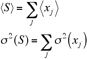
Finally, we can put this together in the equation for a Gaussian probability distribution to get a good approximation for the distribution of S.

The Wilson distribution is the probability distribution for structure factors that applies when we know how many atoms of each type there are in a crystal, but not where those atoms are located. If we know the type of the atom then we know its scattering factor, f, but if we assume that each atom could equally well be anywhere in the unit cell, the phase of its contribution to a structure factor could take any value. The Wilson distribution is useful (for instance) for scaling data and determining the overall thermal motion.
Basically, when we know the identity of the atoms but not their positions, each acentric structure factor is the result of a random walk in the complex plane.
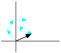
Wilson saw that, because of the central limit theorem, the structure factor distribution for a crystal structure with a sufficient number of atoms would have to be Gaussian. (In fact, the number of atoms does not have to be too large, but the structure shouldn't be dominated by a few heavy atoms.) An exact solution of the probability distribution is very complicated, but a Gaussian approximation is easy to evaluate.
First, we separate the real and imaginary components of the structure factor.
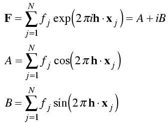
The real and imaginary components of the structure factor are each sums with a term contributed by each atom. We assume that the atoms are independently placed in the unit cell so that the central limit theorem will apply. Then all we need to do is compute the mean and the variance of the real and imaginary parts of the structure factor contributions from each atom. The contribution of an atom must lie somewhere on a circle with radius fj, so we integrate over all phases around that circle.
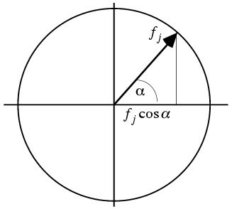
The mean value of either the real or imaginary component will be zero, because the cosine and sine are equally positive and negative. The calculation of the variance is illustrated by integrating the square of the cosine over all possible values of the phase. (The factor of 1/2π expresses a uniform probability for all phase angles.)

Similarly, the integral over the imaginary component gives a value of ½ fj2.
As for the individual atomic contributions, the mean value of the real and imaginary components of the structure factor is zero. The variance of each is the sum of the atomic variances. We define a new parameter, ΣN, to be the sum of the atomic scattering factors squared for all atoms in the structure.
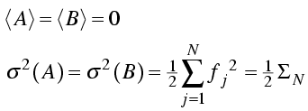
Then we have a simple expression for the probability distributions of the real and imaginary parts of the structure factor.
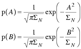
Finally, we assume that the real and imaginary parts of the structure factor are independent, so that their joint distribution (the distribution for the structure factor, F, itself) is the product of the two distributions. This is a two-dimensional Gaussian in the complex plane. (Note that we can substitute the magnitude of the structure factor squared for the sum of the squares of its real and imaginary components.) A common notation for joint probability distributions separates the variables by commas, as in the equation below.
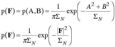
This distribution is illustrated schematically below.
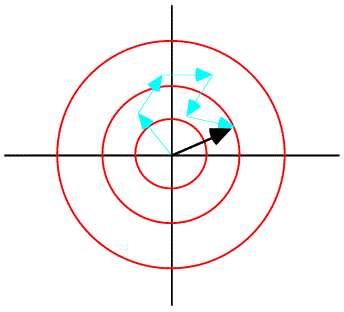
The central limit theorem, as promised, has given us a Gaussian distribution for structure factors. But this distribution is for the structure factors as complex numbers. What we measure in the diffraction experiment is the intensity, which is proportional to the square of the amplitude. To apply the Wilson distribution to amplitudes or intensities, we have to transform variables and integrate out the phase. This changes the form of the distribution, which is no longer Gaussian. We will come back to this in the next lecture.
In the above we have restricted ourselves to acentric structure factors, which form the bulk of a protein data set. For centric structure factors, the contributions from pairs of atoms related by a centre of symmetry are constrained to lie along a line, so we end up with a one-dimensional Gaussian distribution. In small molecule crystallography the difference between the one- and two-dimensional distributions is used to help identify spacegroups, where there can be a choice between a centrosymmetric and non-centrosymmetric alternatives.
We assumed that the contributions of all atoms to the structure factor are independent. This is reasonable for all reflections in the space group P1, but it turns out that symmetry-related atoms do not contribute independently to the structure factor, at least in certain zones of reciprocal space. We will not get into these complications here, but the effect is to change the expected intensity in those zones of reciprocal space. At some point, there will be a Web page that explains this concept in more detail.
Sim asked what we know about a structure factor when we know where some, but not all, of the atoms are. His distribution is actually very much like the Wilson distribution, except that it starts from a known point away from the origin. We can calculate the contribution to the structure factor from the known atoms, which we call FP, and the random walk for the missing or unknown atoms starts at this point in the complex plane, as illustrated schematically below.
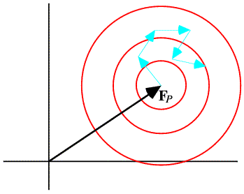
By convention, the missing atoms are called the "Q" atoms. As in the Wilson distribution, each of these atoms contributes ½ fj2 to the variance of the real and imaginary parts. In the case of the Sim distribution, the sum of the scattering factors squared is called ΣQ, and it plays the same role as ΣN in a two-dimensional Gaussian. However, the Gaussian for the Sim distribution is centered on FP. Because it depends on the value of FP, which itself is a random variable, we would say that the Sim distribution is a conditional probability distribution. One notation for such a distribution puts the fixed variables after a semicolon, as in the equation below.

The Sim distribution describes a very artificial case, as it is hard to imagine a situation where we have perfect but incomplete knowledge of a crystal structure. Nonetheless, this distribution turns out to share many features of more realistic, more general distributions.
Rather than work up in complexity, I will start by considering a very general probability distribution, then show how some other distributions arise as special cases of this distribution. We will consider the general problem of the relationship between the structure factors of two isomorphous structures. These are related structures (same space group, similar unit cells, similar atomic contents) that may differ in the identities, occupancies, B-factors or precise positions of the atoms. The two isomorphous structures could indeed represent different crystals (native and heavy-atom derivative, native and ligand-bound) or they could represent the true structure and a model of that structure. So these probability distributions are of wide-ranging relevance.
The effect of differences in position is easiest to consider. Let us assume that there is a probability distribution for differences in the position of each atom, p(xj). This translates into a probability distribution for the contribution of that atom to the overall structure factor; changing the position of the atom changes the phase of its contribution.
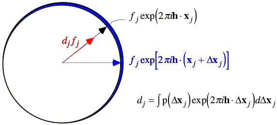
We can find the expected value of the contribution of the atom by integrating over the possible positions of that atom. When we carry out this integration, we average the complex number around a circle, which gives us a complex number inside the circle. The average contribution from the atom will be in the same direction as the original position of the atom, for any reasonable probability distribution. (If it wasn't, then the atom isn't in its most likely position and should be moved in our model!) So the effect of carrying out the integration is to scale down the atomic contribution by a factor dj. Note that the integral to obtain dj is in fact the Fourier transform of the probability distribution of positional differences. Weighting the contribution of the atom by this Fourier transform is equivalent (by the convolution theorem) to smearing the atom out over this distribution of possible positions. (Strictly speaking, we should be treating the real and imaginary parts of the atomic contribution separately, but this way of approaching the problem is more intuitive and ends up being basically correct.)
The variance is computed by considering the possible vector differences between the centroid contribution (red arrow in the figure above) and the possible values of the true value of that contribution (for example, the blue arrow). The probability distributions for these individual atomic deviations are illustrated schematically below: possible values for the vector difference lie on a circle centered on dj fj. These distributions add up to give a two-dimensional Gaussian distribution in the complex plane.

|
Optional advanced material: On average, the contributions of the atoms to the real and imaginary parts of the variance of the 2D Gaussian are given by (1-dj2)fj2/2. This makes sense, if only from the point of view of conservation of scattering matter in the crystal! When the atomic contributions have between weighted down by a factor dj, the Wilson parameter for the distribution of the calculated structure factors will be given by Σdj2fj2. However, the true structure factor must have a Wilson parameter given by Σfj2, and the 2D Gaussian is just the right size to make up the difference. |
Note that this treatment will also handle missing atoms. A missing atom has an essentially infinite uncertainty in its position, so that its contribution to the structure factor can have any phase value; dj is zero.
It turns out that, in general, a wide variety of errors lead to the same kind of two-dimensional Gaussian distribution. In general, if FC is the structure factor computed from a model, the centroid of the probability distribution for the true structure will be obtained by multiplying FC by a parameter D (which arises for similar reasons as dj above). Of course, FC could equally be replaced by (say) the structure factor from an isomorphous crystal.
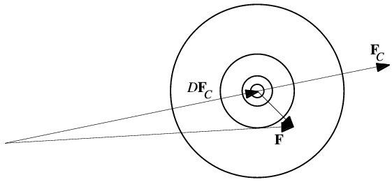
When expressed mathematically, the probability distribution looks very much like the Sim distribution, except that it is centered on DFC. The role of ΣQ is taken by a parameter that depends on D as well as the amount of scattering matter in the model.
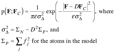
I have included the expected intensity factor, ε, for completeness.
It may help to have an intuitive picture of the meaning of these distributions. We can think of D as the fraction of the structure factor that is correct. Remaining error is random and takes the form of a 2D Gaussian distribution. The width of this Gaussian is sufficient to make up the missing scattering; the smaller D is, the bigger the remaining variance must be.
Similar reasoning can be used to derive a distribution that applies to centric reflections, but we will not go into details here.
The Luzzati distribution, which was derived much earlier, corresponds to a special case of the general distribution. Luzzati assumed that all of the atoms were subject to errors from the same Gaussian distribution of coordinate errors. So dj is the same for all atoms (for any particular reflection) and is equal to D for that reflection. He also assumed that the model was complete. The only difference from the general distribution is that the expression for the variance term can be simplified as follows:
![]()
It should be noted that the basic assumption of the Luzzati distribution is suspect: different atoms will always be subject to different coordinate errors. It is easier to place a well-ordered heavy atom in the structure than a poorly-ordered light one, but the Luzzati distribution assumes they are the same. However, in fairness to Luzzati, he never intended his distributions to be used to estimate coordinate errors!
Although we will not go into detail, the Sim distribution is also a special case of the general distribution given above. In this case the atoms fall into two categories: ones with perfectly known positions (probability distribution is a delta function, dj is one) and ones with unknown positions (probability distribution is infinitely broad, dj is zero).
Srinivasan realised that the Sim and Luzzati distributions could be put into the same form, if the probabilities were expressed in terms of normalised structure factors, or E-values. So, while the Sim distribution treats incomplete but otherwise perfect models and the Luzzati distribution treats complete models with coordinate errors, the Srinivasan distribution treats incomplete models with coordinate errors. In his distribution, like the Sim distribution, the atoms fall into two categories: ones with positions subject to the same Gaussian uncertainty (constant dj for all atoms for a particular reflection) and ones with unknown positions (dj again is zero). The probability distribution is related to the general one, with a change of variables.
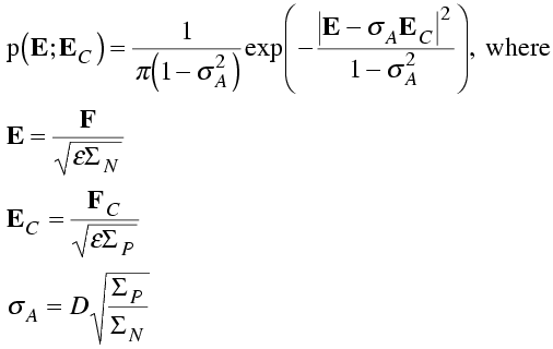
Even when we consider the more general treatment of model errors, the probability distributions have the same form, and it is useful to work with normalised structure factors. The parameters are the same; all that differs is the interpretation we place on them.
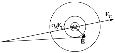
In this distribution, the parameter σA takes the place of D. Like D, σA can be thought of as the fraction of the normalised structure factor that is correct.
The structure factor distributions we have considered so far tell us what we would know about one structure factor if we had measured (or calculated) a related one, but before measuring the amplitude of the structure factor. Once we know the amplitude of the structure factor, only the points in the complex plane with that amplitude are relevant. The measured amplitude defines a circle in the complex plane that cuts through the complex structure factor distribution. By fixing the amplitude in the 2D distribution and normalising (so the overall probability of the phase having some value from 0 to 2π is one), we turn the structure factor probability distribution into a phase probability distribution. This is illustrated schematically in the following figure.
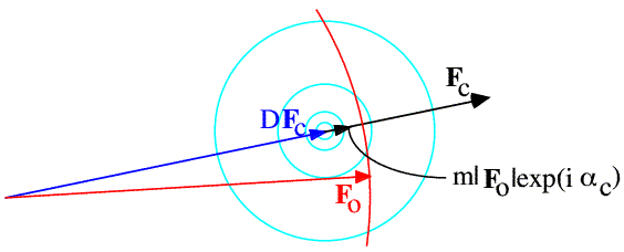
In the case of phases computed from a model, the 2D Gaussian in the complex plane is symmetrical about the model structure factor, so the phase distribution is symmetrical about the model phase and the best phase is always the model phase itself.
The program SIGMAA implements some of this theory about structure factor probabilities to compute Fourier coefficients for model-phased maps. By understanding the phase probability distributions we can compute maps that reduce the random noise from phase error. By understanding the origin of model bias, we can also correct these maps for the predictable bias component.
As discussed above, figure of merit weighting minimises the rms error in an electron density map. But as we realised from considering the implications of Parseval's theorem, the use of model phases will introduce bias for the map to resemble the model more than it should. (Remember, in the complex plane the model-phased structure factor is closer to the model structure factor than the true structure factor is.)
The reduction of model bias in SIGMAA generalises early ideas that missing atoms and extra atoms in the model both tend to show up at half height. Peter Main treated the case where the map coefficients are weighted by figures of merit derived from the Sim distribution. Applying his results to the more general distributions just requires a change of variables. The basic outline of the derivation will be given below.
First we start with the cosine law.
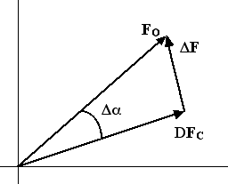
![]()
Taking the expected value of each side of this equation introduces the figure of merit.
![]()
With further manipulations (not reproduced here), we can solve for a figure-of-merit weighted Fourier coefficient, which shows that the resulting map will have features of both the true structure and the model, both at half height.

Now we can solve for an approximation to the true structure factor, which eliminates the predictable bias component of the figure-of-merit weighted map coefficient.
![]()
Maps computed from these coefficients generally do seem to suffer significantly less from model bias. At the least, they make it more obvious where the model is wrong, even if the correct interpretation is not always clear.
The theory of map coefficients for maps combining phase information from different sources is less clear. SIGMAA makes the approximation that the amount of model bias in a figure-of-merit weighted map coefficient, computed with combined phases, depends directly on the model's influence on the combined phase. In other words, it is assumed that the combined phase map coefficient is a linear combination of the coefficients that would be obtained through MIR and model phases alone.
If all the phase information comes from experimental phases such as MIR, there is no model bias, just random noise. We have already seen the bias component introduced by model phases.
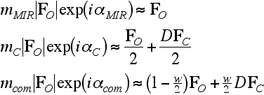
We are assuming here that phase combination gives the linear combination of MIR and model phases. But we need some measure of the extent to which the model phases have influenced the combined phase. Information theory gives an intuitively reasonable answer: the relative influence of the two sources of phase information depends on the relative information content of their phase probability distributions.
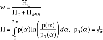
Finally, having determined the weighting factor, we can solve for an approximation to the true structure factor. You can see, by inspecting this equation, that it reduces to an appropriate expression when all the phase information comes from one source, either MIR or a model.

Although the derivation of these combined-phase map coefficients is far from rigorous, the result is intuitively reasonable and, in practice, the maps give good results.
The program SIGMAA reads in a file containing the observed and calculated structure factor amplitudes and the calculated phases, and computes phase probability distributions. The calculations are done by maximising a likelihood function, which will be explained in a bit more detail in the next lecture.
The program can also optionally read in prior experimental phase information, in the form of Hendrickson-Lattman coefficients, A, B, C, D. These describe the prior phase information according to the following formula:
![]()
Then various types of map coefficient can be computed.

Finally, the program can produce data for a σA plot, which can be interpreted (according to the Srinivasan distribution) in terms of model completeness and mean-square coordinate error. This is based on the same theory as the Luzzati plot, but with fewer assumptions. Such overall measures of coordinate error should be taken as a rough guide only, because the remaining necessary assumptions are poorly-founded. Most seriously, these plots depend on coordinate errors being independent of atom type or thermal motion. But of course the heaviest and most well-ordered atoms will suffer much less from errors than the lightest and most poorly-ordered atoms.
© 1999-2009 Randy J Read, University of Cambridge. All rights reserved.
Last updated: 6 April, 2009