
|
Protein Crystallography Course
|
One of the most important concepts in Fourier theory, and in crystallography, is that of a convolution. Convolutions arise in many guises, as will be shown below. Because of a mathematical property of the Fourier transform, referred to as the convolution theorem, it is convenient to carry out calculations involving convolutions.
But first we should define what a convolution is. Understanding the concept of a convolution operation is more important than understanding a proof of the convolution theorem, but it may be more difficult!
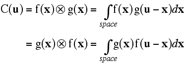
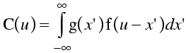
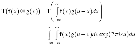
Mathematically, a convolution is defined as the integral over all space of one function at x times another function at u-x. The integration is taken over the variable x (which may be a 1D or 3D variable), typically from minus infinity to infinity over all the dimensions. So the convolution is a function of a new variable u, as shown in the following equations. The cross in a circle is used to indicate the convolution operation.
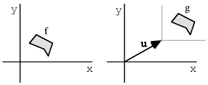
Note that it doesn't matter which function you take first, i.e. the convolution operation is commutative. We'll prove that below, but you should think about this in terms of the illustration below. This illustration shows how you can think about the convolution, as giving a weighted sum of shifted copies of one function: the weights are given by the function value of the second function at the shift vector. The top pair of graphs shows the original functions. The next three pairs of graphs show (on the left) the function g shifted by various values of x and, on the right, that shifted function g multiplied by f at the value of x.
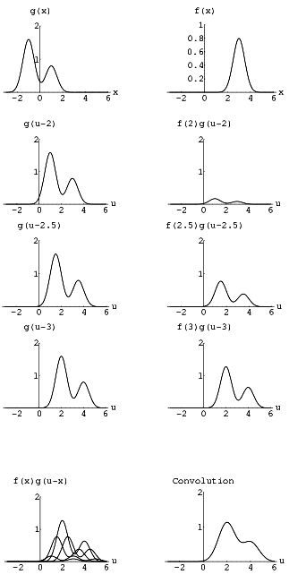
The bottom pair of graphs shows, on the left, the superposition of several weighted and shifted copies of g and, on the right, the integral (i.e. the sum of all the weighted, shifted copies of g). You can see that the biggest contribution comes from the copy shifted by 3, i.e. the position of the peak of f.
If one of the functions is unimodal (has one peak), as in this illustration, the other function will be shifted by a vector equivalent to the position of the peak, and smeared out by an amount that depends on how sharp the peak is. But alternatively we could switch the roles of the two functions, and we would see that the bimodal function g has doubled the peaks of the unimodal function f.
![]()
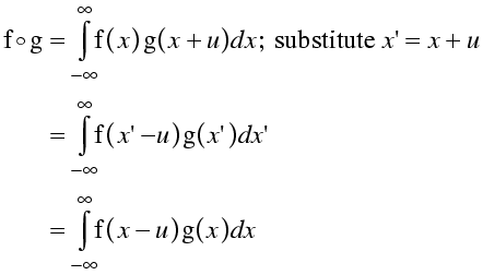
We stated that the convolution integral is commutative. Here, in case you are interested, is a quick proof of that. First, we start with the convolution integral written one way. For convenience we will deal with the 1D case, but the 3D case is exactly analogous.
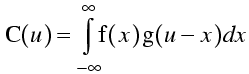
Now we substitute variables, replacing u-x with a new x'.
![]()
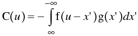
Note that, because the sign of the variable of integration changed, we have to change the signs of the limits of integration. Because these limits are infinite, the shift of the origin (by the vector u) doesn't change the magnitude of the limits.
Now we reverse the order of the limits, which changes the sign of the equation, and swap the order of the functions g and f.
It doesn't matter whether we call the variable of integration x' or x, so we put back x, to get the result we wanted to prove.
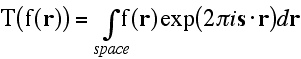
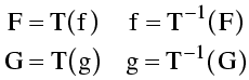
Because there will be so many Fourier transforms in the rest of this presentation, it is useful to introduce a shorthand notation. T will be used to indicate a forward Fourier transform, and its inverse to indicate the inverse Fourier transform.
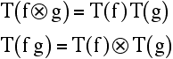
There are two ways of expressing the convolution theorem:
The convolution theorem is useful, in part, because it gives us a way to simplify many calculations. Convolutions can be very difficult to calculate directly, but are often much easier to calculate using Fourier transforms and multiplication.
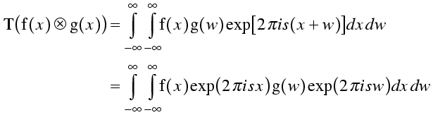
To prove the convolution theorem, in one of its statements, we start by taking the Fourier transform of a convolution. What we want to show is that this is equivalent to the product of the two individual Fourier transforms. Note, in the equation below, that the convolution integral is taken over the variable x to give a function of u. The Fourier transform then involves an integral over the variable u.
Now we substitute a new variable w for u-x. As above, the infinite integration limits don't change. Then we expand the exponential of a sum into the product of exponentials and rearrange to bring together expressions in x and expressions in w.
Expressions in x can be taken out of the integral over w so that we have two separate integrals, one over x with no terms containing w and one over w with no terms containing x.
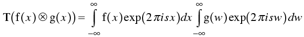
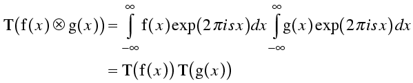
The variables of integration can have any names we please, so we can now replace w with x, and we have the result we wanted to prove.
If you look through the derivation above, you will see that we could have used a minus sign in the exponential when taking the original Fourier transform, and then the two Fourier transforms at the end would also contain minus signs in the exponentials. In other words, the convolution theorem applies to both the forward and reverse Fourier transforms. This is not surprising, since the two directions of Fourier transform are essentially identical.
To prove the second statement of the convolution theorem, we start with the version we have already proved, i.e. that the Fourier transform of a convolution is the product of the individual Fourier transforms.
![]()
First we'll define some shorthand, where capital letters indicate the Fourier transform mates of lower case letters.
We use these relationships to recast the statement above in terms of the Fourier tranform mates of the original functions. Then we take an inverse Fourier transform on each side of the equation, to get (essentially) the second statement of the convolution theorem. The only difference is that it is expressed in terms of the inverse Fourier transform.
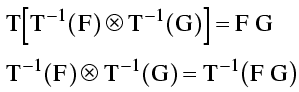
But, as we noted above, we could have proved the convolution theorem for the inverse transform in the same way, so we can reexpress this result in terms of the forward transform.
![]()
The correlation theorem is closely related to the convolution theorem, and it also turns out to be useful in many computations. The correlation theorem is a result that applies to the correlation function, which is an integral that has a definition reminiscent of the convolution integral.
In a correlation integral, instead of taking the value of one function at u-x, you take the value of that function at x-u. Equivalently, you take the value of the other function at x+u. This is shown in the following equation, along with the variable substitution that allows the two expressions to be interconverted.
The figure below illustrates why the correlation function has the name that it does. If the two functions f and g contain similar features, but at a different position, the correlation function will have a large value at a vector corresponding to the shift in the position of the feature.
The correlation theorem can be stated in words as follows: the Fourier tranform of a correlation integral is equal to the product of the complex conjugate of the Fourier transform of the first function and the Fourier transform of the second function. The only difference with the convolution theorem is in the presence of a complex conjugate, which reverses the phase and corresponds to the inversion of the argument u-x.
![]()
First we need to define a Gaussian function. We will stick, for the moment, to 1D Gaussians. The Gaussian function is the familiar bell-shaped curve, with a peak position (r0) and standard deviation.
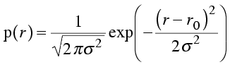
We won't derive the Fourier transform of a Gaussian, but it is given by the following equation.
Note that the Fourier transform of a Gaussian is another Gaussian (although lacking the normalisation constant). There is a phase term, corresponding to the position of the center of the Gaussian, and then the negative squared term in an exponential. Also notice that the standard deviation has moved from the denominator to the numerator. This means that, as a Gaussian in real space gets broader, the corresponding Gaussian in reciprocal space gets narrower, and vice versa. This makes sense, if you think about it: as the Gaussian in real space gets broader, contributions from points within that Gaussian start to interfere with each other at lower and lower resolutions.
Convolution with a Gaussian will shift the origin of the function to the position of the peak of the Gaussian, and the function will be smeared out, as illustrated above.
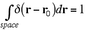
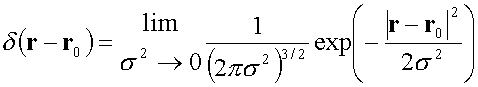
Delta functions have a special role in Fourier theory, so it's worth spending some time getting acquainted with them. A delta function is defined as being zero everywhere but for a single point, where it has a weight of unity.

What it means to say that it has a weight of unity is that the integral of the delta function over all space is 1. The delta function is given an argument of r-r0 so that it can be defined as having its non-zero point at the origin. When r is equal to r0, the argument of the delta function is zero.
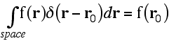
A more general property of the delta function is that the integral of a delta function times some other function is equal to the value of that other function at the position of the delta function.
How can a single point, with no width, breadth or depth, have a weight of one? The value of the delta function at that point must be a special kind of infinity, and this means that it has to be defined as a limit. There are a number of ways to define a delta function. One of them is to define it as an infinitely sharp Gaussian. The integral over all space of a Gaussian is 1, which satisfies one of the properties required for the delta function, and if we take the limit of a Gaussian as the standard deviation tends to zero, it satisfies the other properties. The following equation defines a 3D delta function as the limit of an isotropic 3D Gaussian.
With this definition of the delta function, we can use the Fourier transform of a Gaussian to determine the Fourier transform of a delta function. As the standard deviation of a Gaussian tends to zero, its Fourier transform tends to have a constant magnitude of 1. All that is left is the phase shift term.
![]()
So we see that the Fourier transform of a delta function is just a phase term. Think about the picture we had of an electron at a point; it contributed just a phase term, with unit weight, to the diffraction pattern. So now we see that we can consider an electron at a point to be a delta function of electron density.
Finally we can consider the meaning of the convolution of a function with a delta function. If we write down the equation for this convolution, and bear in mind the property of integrals involving the delta function, we see that convolution with a delta function simply shifts the origin of a function.

![]()
We have essentially seen this before. We can tabulate atomic scattering factors by working out the diffraction pattern of different atoms placed at the origin. Then we can apply a phase shift to place the density at the position of the atom. Our new interpretation of this is that we are convoluting the atomic density distribution with a delta function at the position of the atom.
We can think of thermal motion as smearing out the position of an atom, i.e. convoluting its density by some smearing function. The B-factors (or atomic displacement parameters, to be precise) correspond to a Gaussian smearing function. At resolutions typical of protein data, we are justified only in using a single parameter for thermal motion, which means that we assume the motion is isotropic, or equivalent in all directions. (In crystals that diffract to atomic resolution, more complicated models of thermal motion can be constructed, but we won't deal with them here.)
Above, we worked out the Fourier transform of a 1D Gaussian.
In fact, all that matters is the displacement of the atom in the direction parallel to the diffraction vector, so this equation is suitable for a 3D Gaussian. All we have to remember is that the term corresponding to the standard deviation refers only to the direction parallel to the diffraction vector. Since we are dealing with the isotropic case, the standard deviation (or atomic displacement) is equal in all directions.
The B-factor is used in an equation in terms of sinθ/λ instead of the diffraction vector, because all that matters is the magnitude of the diffraction vector. We replace the variance (standard deviation squared) by the mean-square displacement of the atom in any particular direction. The B-factor can be defined in terms of the resulting equation.
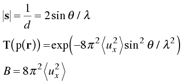
Note that there is a common source of misunderstanding here. The mean-square atomic displacement refers to displacement in any particular direction. This will be equal along orthogonal x, y and z axes. But often we think of the mean-square displacement as a radial measure, i.e. total distance from the mean position. The mean-square radial displacement will be the sum of the mean-square displacements along x, y and z; if these are equal it will be three times the mean-square displacement in any single direction. So the B-factor has a slightly different interpretation in terms of radial displacements.
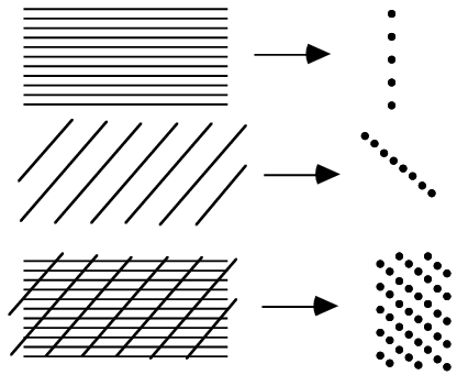
The convolution theorem can be used to explain why diffraction from a lattice gives another lattice – in particular why diffraction from a lattice of unit cells in real space gives a lattice of structure factors in reciprocal space. The Fourier transform of a set of parallel lines is a set of points, perpendicular to the lines and separated by a distance inversely proportional to the space between the lines. (This is related to the idea that diffraction from a set of Bragg planes can be described in terms of a diffraction vector in reciprocal space, perpendicular to the set of planes. In fact, we can increase "n" in Bragg's law (nλ=2 d sinθ) to get a series of diffraction vectors for that set of planes.) In the figure below, one set of closely-spaced horizontal lines gives rise to a widely-spaced vertical row of points. A second set of more widely-space diagonal lines gives rise to a more closely-spaced row of points perpendicular to these lines. If we multiply one set of lines by another, this will give an array of points at the intersections of the lines in the bottom part of the figure. The Fourier transform of this lattice of points, which was obtained by multiplying two sets of lines, is the convolution of the two individual transforms (i.e. rows of points) , which generates a reciprocal lattice.
Of course, the same argument can be applied to a 3D lattice.
A crystal consists of a 3D array of repeating unit cells. Mathematically, this can be generated by taking the content of one unit cell and convoluting it by a 3D lattice of delta functions. The diffraction pattern is thus the product of the Fourier transform of the content of one unit cell and the Fourier transform of the 3D lattice. Since the transform of a lattice in real space is a reciprocal lattice, the diffraction pattern of the crystal samples the diffraction pattern of a single unit cell at the points of the reciprocal lattice.
Truncating the resolution of the data used in calculating a density map is equivalent to taking the entire diffraction pattern and multiplying the structure factors by a function which is one inside the limiting sphere of resolution and zero outside the limiting sphere. The effect on the density is equivalent to taking the density that would be obtained with all the data and convoluting it by the Fourier transform of a sphere. Now, the Fourier transform of a sphere has a width inversely proportional to the radius of the sphere so, the smaller the sphere (i.e. the lower the limiting resolution), the more the details of the map will be smeared out (thus reducing the resolution of the features it shows). In addition, the Fourier transform of a sphere has ripples where it goes negative and then positive again, so a map computed with truncated data will also have Fourier ripples. These will be particularly strong around regions of high density, such as heavy atoms.
Similarly, leaving out any part of the data set (e.g. if you are missing a wedge of data in reciprocal space because the crystal died before the data collection was finished, or you didn't collect the cusp data) will lead to distortions of the electron density that can be understood through the convolution theorem. As for resolution truncation, missing data can be understood as multiplying the full set of data by one where you have included data and zero where it is missing. The convolution theorem tells us that the electron density will be altered by convoluting it by the Fourier transform of the ones-and-zeros weight function. The more systematic the loss of data (e.g. a missing wedge versus randomly missing reflections), the more systematic the distortions will be.
The presentation on density modification shows that the effect of solvent flattening can be understood in terms of the convolution theorem. The effect of solvent flattening is that each structure factor after solvent flattening is obtained by taking the weighted average of its neighbours (in the reciprocal lattice) before solvent flattening, with the weighting terms being obtained as the Fourier transform of the mask around the protein. So the smaller the protein mask (i.e. the bigger the solvent fraction), the wider the features of its Fourier transform and thus the more widely the new phases consult the old phases in the surrounding region of reciprocal space. Similarly, if the mask is more detailed, then its Fourier transform spreads more widely in reciprocal space and there is more mixing of phase information.
The same presentation shows that Sayre's equation can be considered as an extreme case of solvent flattening, in which every atom provides its own mask.
The Patterson function is simply the correlation function of the electron density with itself. By the correlation theorem, this correlation is computed by taking the Fourier transform of F times its complex conjugate F*, i.e. the Fourier transform of |F|2. At positions in the Patterson map corresponding to vectors between peaks of density in the electron density map, there will be peaks because the relative translation of the two maps in the correlation function will place one peak on top of the other.
The phased translation function is the correlation of one density map with another, as a function of a translation shift applied to one of the maps. This can be computed, using the correlation theorem, by taking the Fourier transform of the structure factor for one map times the complex conjugate of the structure factor for the other map, i.e. by subtracting the phases. Details are given in the presentation on molecular replacement.
© 1999-2009 Randy J Read, University of Cambridge. All rights reserved.
Last updated: 9 April, 2009