
|
Protein Crystallography Course
|
In the second lecture on advanced diffraction, we explored different ways of expressing diffraction, in terms of electron density or atoms, and in terms of diffraction vectors (reciprocal space) or the reciprocal lattice. For our purposes today, the most useful way of thinking of the structure factor equation expresses it in terms of electron density and the reciprocal lattice:
(The integral is carried out over volume elements dv, over the unit cell.) As discussed before, the Miller indices h [=(h k l)] can be thought of in two ways: they specify the Bragg planes that cut the unit cell edges h, k and l times, respectively; they also specify a vector in reciprocal space perpendicular to these planes, with length equal to the reciprocal of the spacing between the Bragg planes. The amplitude |F(h)| of a particular structure factor indicates the extent to which the electron density is concentrated on planes parallel to the Bragg planes, while its phase indicates the position of planes of high electron density relative to the Bragg planes. As we will see below, you can think of each structure factor as expressing the best approximation of the electron density in terms of a single cosine wave.
As mentioned before, the structure factor equation is a Fourier transform, which is a mathematical operation that has been studied for over a century. One of the most useful properties of the Fourier transform is that it is its own inverse: if you apply a Fourier transform twice, you get the original function back. In the inverse Fourier transform, the only difference is that the a negative sign is included in the exponential, and (depending exactly on how the first Fourier transform was defined), there may be a scale constant.
So we can regenerate the electron density from the structure factors with an inverse Fourier transform. The equation is called the electron density equation. In general, an inverse Fourier transform would involve an integral like the forward Fourier transform, but if the object is periodic (like a crystal), it involves just a summation. (As we have seen, diffraction from a crystal cancels out in all directions, except those specified by integer Miller indices.)
In this equation, we have to divide by the volume of the unit cell to recover the electron density on the correct scale. You can understand this intuitively by thinking about the F(000) term, where h, k and l are all zero. In the structure factor equation, F(000) will be equal to the number of electrons in the unit cell. In the electron density equation, F(000) should contribute the average density over the cell to all points in the cell, which means we have to divide by V.
NB: It's important to remember that the electron density equation, as written here, requires us to take a sum over all structure factors in reciprocal space. Because of limited resolution, this will generally be a sphere in reciprocal space. We will see that symmetry in reciprocal space (space group symmetry and Friedel's law) will reduce the number of structure factors we have to consider, if the equation is modified appropriately.
The easiest way to prove the electron density equation is to show that the successive application of the electron density and structure factor equations regenerates the structure factors. If we use the structure factors, F, to calculate electron density in the electron density equation, then calculate new structure factors with the structure factor equation, the new structure factors (which we will call G for the moment) should be equal to the old ones. So first we take the structure factor equation and substitute the electron density equation for the density values.
Note the use of h', because the sum in the electron density equation has to be computed with all structure factors, not just the one (h) we are using in the structure factor equation. If the electron density equation is true, we should find that G(h) = F(h) for all h.
First we combine the exponentials.
Now we rearrange the order of integration and summation to get just the exponential inside the integral.
When h' is not equal to h, the components of (h-h') will be non-zero integers. The integral is taken over the cell, with the x, y and z fractional coordinates varying from 0 to 1. So the argument of the exponential will vary over a whole number of cycles of 0 to 2π. Both the cosine (real) and sine (imaginary) components of the integral will disappear, because cosine and sine are equally positive and negative over a cycle. This is illustrated in the following picture, with positive regions of the integral shaded blue and negative regions shaded orange.
Only the term with h' equal to h will remain. In this case, the argument of the exponential will be zero and exp(0) is 1, so the integral evaluates to the volume of the unit cell. So we are only left with the equation G(h) = F(h), which is what we set out to prove!
It's worth taking some time to understand this proof, because the same kinds of manipulations occur time and again in Fourier theory, particularly in the convolution and correlation theorems (the basis for the Patterson function). The integral disappears because terms with different values of h are (as a mathematician would say) orthogonal to one another. This orthogonality is a very useful feature. One consequence is that, if you are missing one of the structure factors, you don't have to change the values you are using for the other structure factors to compensate.
In the electron density equation, we take the sum of products of one complex number (structure factor) with a complex exponential. So why is the resulting electron density real instead of complex valued? A flippant answer is that electron density is real because we have assumed that it is real!
The assumption that electron density is real has come in when we said that an electron at the origin scatters with a scattering factor of 1e, a real number. In fact, we are defining a phase of zero as the phase of scattering of a "normal" electron from the origin. What we have really assumed, then, is that all electrons are "normal" electrons that diffract with the same relative phase angle. As discussed previously, when we were considering basic aspects of phasing using anomalous scattering, the assumption that all electrons diffract with the same relative phase leads to Friedel's law.
F(h) = F*(-h)
The asterisk indicates the complex conjugate, in which the sign of the imaginary component (or the phase) has been reversed. In other words the reflections at h and -h have the same amplitudes but opposite phases. Another way to look at this, as illustrated below, is that the phase differences for scattering from two sides of the Bragg planes have the same size but opposite signs.
So we can pair up the contributions of Friedel mates in the electron density equation and, as we will see shortly, eliminate the imaginary components.
The sum over a sphere in reciprocal space is replaced by the sum over a hemisphere omitting the origin term. Friedel's law tells us that we can make the following substitutions:
Putting this in the electron density equation, we get:

Now we expand the exponentials with Euler's equation:
When we make the substitution, the imaginary terms cancel.
If an electron has a transition energy close to the energy of an X-ray photon, there will be a phase shift in its contribution to scattering, which is called anomalous scattering. The phase shift means that the scattering factor is represented as having an imaginary component. In these circumstances, as we showed in the phasing lecture, Friedel's law no longer holds. We won't go into the details here, but if you allow for anomalous scatterers and calculate the electron density with all structure factors, the electron density will have an imaginary component at the position of the anomalous scatterers.
By combining the contributions of Friedel mates, we have obtained a form of the electron density equation that has a simple physical interpretation. Each structure factor can be seen to add a single cosine wave to the picture of the electron density. As we know from our study of the structure factor equation, the amplitude of each structure factor tells us the extent to which electrons are concentrated on planes parallel to the Bragg planes. The phase tells us where these concentrations are found.
You can explore the effect of single structure factors, combinations of structure factors, and changes in their amplitudes or phases most easily by playing around with Kevin Cowtan's Interactive Structure Factor Tutorial.
As we've seen, when we measure the diffraction pattern, this gives us only intensities (which can be turned into amplitudes) but not phases for the structure factors. People often say that we only get half of the information we need to calculate an electron density map. In fact, the situation is even worse! The phases are far more important for determining the electron density than the amplitudes are.
The following picture gives a particularly dramatic illustration of the importance of phase. On the top are photographs of Jerome Karle (left) and Herb Hauptman (right), who won the Nobel Prize for their work on solving the phase problem for small molecule crystals. We can treat the photographs as density maps and calculate their Fourier transforms, to get amplitudes and phases.
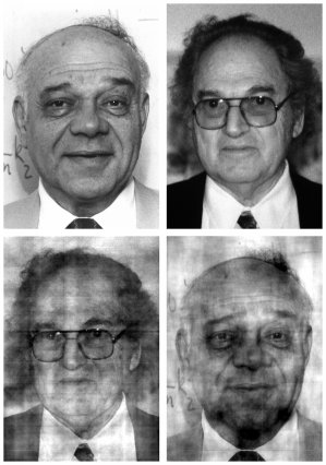
If we combine the phases from the picture of Hauptman with the amplitudes from the picture of Karle, we get the picture on the bottom left. The bottom right picture combines the phases of Karle with the amplitudes of Hauptman. Clearly the phases are dominating what we see. This is terribly worrying when we consider using phases from an atomic model.
Fortunately, it turns out that the situation is not quite as grim when the model is closer to reality than in this extreme example. But we still need to worry about model bias.
Often we can understand what we see in an electron density map and why we see it by considering Parseval's theorem, which is an important basic result in Fourier theory. Parseval's theorem says, in words, that the mean-square value on one side of the Fourier transform is proportional to the mean-square value on the other side of the Fourier transform.
In a later lecture, when we consider the convolution and correlation theorems, we will see that Parseval's theorem arises as a trivial special case. The mean-square density is obtained by dividing the integral by the unit cell volume V, so:
More simply, the rms density is proportional to the rms structure factor amplitude.
![]()
Fourier transforms are additive (we've been assuming that all along, in adding up the contributions of electrons or atoms), so the same relationship applies to difference density.
![]()
Note that the structure factor difference is a vector difference between the complex numbers, including their phases.
Now we can understand how the phases dominated the photos of Karle and Hauptman. If we make a random choice of phase, the rms error that is introduced in the structure factor is greater than the structure factor itself, which means that a flat map would be a better picture of the true structure. On the other hand, a random choice of amplitude introduces a much smaller rms error; in fact, the error that is introduced is smaller than the typical structure factor, so that a map with true phases but random (or mismatched) amplitudes still looks like the object that contributed the phases. This is illustrated schematically in the following picture.
Many structures are solved by molecular replacement, so there is never any phase information other than the phases that can be computed from an atomic model. Even when there is experimental phase information, the model phases generally become much more accurate than the experimental phases towards the end of refinement. So we are often looking at maps that combine (in some way--more on this later) observed amplitudes with model phases.
Given the overwhelming importance of the phase, how do model-phased maps tell us anything about the structure? The following schematic figure allows us to understand, through Parseval's theorem, why such maps show features that are not in the model.
We can measure the amplitude of the true structure factor, F, but not its phase, so we know that it lies somewhere on a circle. The structure factor calculated from a model, FC, can be used to supply a phase, giving the structure factor that combines the observed amplitude with the calculated phase, |F|exp(iαC). This model-phased structure factor is closer to the true F than FC was, so the corresponding map will have features of the true structure that were not in the model. So, for instance, if some atoms are missing from the model, they will still show up in the model-phased density map.
In the figure above, we can also see that the model-phased structure factor, |F|exp(iαC), is also closer to the calculated structure factor, FC, than the true structure factor, F, was. So the corresponding map will also have features of the model that are not in the true map.
Since the model-phased map shows features of the true structure that are not in the model, one way to highlight these features is to subtract the model map from the model-phased map. Because the Fourier transform is additive, this is achieved by simply subtracting the structure factors: (|F|-|FC|)exp(iαC).
We can also understand this map as follows. Part of the true (complex) difference between F and FC will be in the direction of FC, i.e. in the direction of the difference structure factor used in the map. This will show up true features of the difference between the true structure and the model. Part of the true difference will be out-of-phase, or perpendicular to FC, and its contribution will be lost because we don't know the direction of the phase error. If there are only small differences between the model and the true structure, it turns out that the in- and out-of-phase components are about half and half, so that the difference map shows the differences at half height.
According to Parseval's theorem, the rms error in the electron density map is proportional to the rms error in the (complex) structure factor. So to minimise the rms error in our electron density, we should find the structure factor that minimises the rms error in the complex plane. Blow and Crick showed that, if we know something about the probabilities of different possible phase choices, we can minimise the rms error in the structure factor by taking its probability-weighted average over all possible phase choices.
The process of taking a probability-weighted average is illustrated in the figure below. The circle represents possible values for the complex structure factor F, with its different possible phase choices. The probability of each possible phase is indicated by the thickness of the blue line around the circle. Averaging a complex number around a circle gives a complex number inside the circle, i.e. one with a smaller magnitude than the radius of the circle. This average complex number also has a phase, which Blow and Crick termed the "best phase". The reduction in the amplitude is expressed through a number called the figure of merit, m. For perfect phase information, the figure of merit is 1. As the phase information becomes more ambiguous, the figure of merit drops, until it becomes zero when all phases are equally probable.
We'll hear a lot more about figures of merit and optimal structure factors to use for maps (also called "map coefficients") later, when we have covered more background theory on phase probabilities.
© 1999-2009 Randy J Read, University of Cambridge. All rights reserved.
Last updated: 26 February, 2010