Protein Crystallography Course

Advanced diffraction:
atoms, crystals and reciprocal space

This page is a revised version of the second half of basic diffraction theory, aimed at a deeper understanding of the mathematics and physics.

Outline

• When do we see diffraction from a crystal?
• Reciprocal space
  • The reciprocal lattice
  • Structure factors in terms of atoms
  • The Ewald sphere
  • Diffraction from a real crystal
• Quantum mechanics and diffraction
• Other resources

When do we see diffraction from a crystal?

As we have mentioned before, a crystal amplifies the diffraction pattern in certain directions, where the various unit cells diffract in phase, and eliminates it in other directions. In order for the unit cells to diffract in phase, the Bragg planes must pass through the same points in all the unit cells in the crystal. The easiest case to imagine is when the planes are separated by one unit cell edge, or an integral fraction of a unit cell edge. In the following picture, you can see that sets of planes separated by one unit cell edge or one-third unit cell edge will pass through equivalent atoms in the different unit cells. On the other hand, if the planes divide the unit cell edge by a non-integral number, the different unit cells will all diffract out of phase and the waves will cancel out.

The black lines in the figure outline the unit cells, the red lines indicate planes separated by one unit cell edge along the a cell axis, and the blue lines indicate planes separated by one-third unit cell edge along a.

Note on indexing diffraction patterns with Miller indices: the red planes are called the (1 0 0) planes because they divide the a cell edge once, and the blue planes are called the (3 0 0) planes because they divide the a cell edge three times. This again relates to the idea of reciprocal space: the planes (and corresponding diffraction spots) with larger indices correspond to closer spacings; the (3 0 0) planes are one-third as far apart as the (1 0 0) planes. The three indices are called h, k and l, so that in the figure above we are looking at two sets of (h 0 0) planes.

In general, to see diffraction from a crystal, the Bragg planes have to cut all the cell edges an integral number of times. (In, say, the (3 0 0) planes, the b and c cell edges are cut zero times.) It's easier to illustrate this in only two dimensions by looking at (h k 0) planes. Three sets of these are shown in the figure below.

This is a bit more complicated! First look at the blue planes. As we follow the blue arrow from one plane to the next, the next plane is one unit cell further along in both the a and b directions, so these are the (1 1 0) planes. The magenta planes are similar, but as we follow the magenta arrow from one plane to the next, the next plane is one cell edge further in the a direction, but one cell edge back in the b direction, so these are the (1 -1 0) planes. With the green planes, as we follow the green arrow from one plane to the next we move half a unit cell edge along a and a full cell edge along b, so these are the (2 1 0) planes. (Another way to look at this is that we have to cross two planes to move one cell edge along a but only one plane to move one cell edge along b.)

Reciprocal space

We have mentioned different ways in which the concept of reciprocal space arises: higher angle scattering corresponds to closer spacings; increasing the indices of the planes corresponds to finer sampling along the cell edges. However, mathematically, reciprocal space is the space defined by the diffraction vectors, s. These diffraction vectors, as illustrated in the last lecture, are perpendicular to their corresponding Bragg planes and their length is inversely proportional to the d-spacing between those planes.

The space of diffraction vectors, s, is also the inverse space created by application of the Fourier transform to the electron density defined over real space, r.

The reciprocal lattice

We've just seen one way to think about reciprocal space: the Miller indices (h k l) that define Bragg planes allowing diffraction (constructive interference) from a crystal. In the last lecture, we looked at the diffraction vector s, a vector perpendicular to the Bragg plane with a length equal to the reciprocal of the interplanar spacing. It is useful to consider the relationship between these ways of defining planes and reciprocal space. It turns out that the Miller indices provide a useful way to define reciprocal lattice points within the reciprocal space defined by s. We will see that the reciprocal lattice is defined by a reciprocal unit cell, in the same way that the crystal lattice is defined by the crystal (real space) unit cell.

We will define the reciprocal unit cell by the three diffraction vectors corresponding to planes separated by the three real-space unit cell axes. Let's think first about the a axis. The (1 0 0) planes are separated by integral multiples of a. You might think that the corresponding diffraction vector s should be parallel to a, but that is not necessarily true. The Bragg planes are defined by the b and c axes, so the diffraction vector must be perpendicular to the bc plane. As you can see in the figure below, for a non-orthogonal unit cell a is not necessarily perpendicular to the bc plane. We define the first reciprocal cell axis, called a*, as the diffraction vector for the (1 0 0) planes. Its length is the reciprocal of the distance between one bc plane and the next, and it is perpendicular to the bc plane. The figure below shows a section through a monoclinic unit cell, where only the angle β is non-orthogonal. (When we study symmetry, we will learn about different crystal classes and how different symmetries impose different restrictions on the unit cells.)

The (3 0 0) planes are separated by one-third of the spacing between bc planes, so the diffraction vector is three times as long and is therefore equivalent to 3a*. In general, the diffraction vector for any (h 0 0) set of planes is given by ha*. The other two reciprocal axes are defined analogously. So any point in the reciprocal lattice can be defined as the sum of integral multiples of the reciprocal axes:

s = ha* + kb* + lc*

When we describe points in the reciprocal lattice with Miller indices (h k l), it turns out to be useful (for reasons that will become immediately obvious) to describe positions in real space with fractional coordinates, (x y z). The fractional coordinates are defined as fractions of the unit cell axes, so that we express a position r as:

r = xa + yb + zc

This is illustrated in the following picture, together with the direction of a*:

The reason this is useful is because the Miller indices implicitly incorporate the cell dimensions in such a way that we can now replace the dot product s·r with h·x.

The simplifications occur because of the relationships between the real and reciprocal axes discussed above, where the dot products simplify to 1 for pairs such as a and a* and to 0 for pairs such as a and b*.

This now allows us to express the structure factor equation in terms of Miller indices and fractional coordinates.

Note that the integral is now being taken only over a single unit cell. That is because taking it over a larger number of unit cells would simply multiply the structure factor by the number of unit cells. By convention, the structure factor is defined as the Fourier transform of a single unit cell.

Structure factors in terms of atoms: the atomic scattering factor

We now have the structure factor equation expressed in terms of Miller indices, which relate to the individual spots we observe in a diffraction pattern. However, when we build a model we will be working with atoms, not directly with their electron density distributions. So the next useful step is to express the structure factor equation in terms of the types and positions of individual atoms.

Remember that the structure factor equation was derived first as the sum of contributions from individual electrons, so we can break it up into the sum of contributions from the electrons comprising individual atoms. (Another way to say this is that the Fourier transform of a sum is the sum of the individual Fourier transforms.)

Next, remember that the contribution of an electron at the origin to the structure factor was 1e, with a phase of zero, for all diffraction vectors. Moving the atom to a different point in the unit cell just changed the phase of its contribution in a way that depended on both its position (r) and the diffraction vector (s): the new phase was given by 2πs·r. In the same way, we might expect that we could calculate the contribution to the structure factor of an atom at the origin and then change its phase according to its position in the unit cell. However, we can also derive such a result quite simply from scratch, as shown below.

Since the diffraction pattern of an atom centered on the origin depends only on the type of atom, we can tabulate it before hand. To a very good approximation, we can consider the electron density of an atom centered on the origin to be spherically symmetric. This has two consequences:

1. the phase of its overall scattering will be zero, because for any electron density at +r there will be equal electron density at -r, which will cancel out any imaginary contribution.

2. its diffraction will depend only on resolution (|s|) and not on the direction of the diffraction vector.

At very low scattering angles (corresponding to d-spacings much wider than the dimensions of the atom), the electrons of the atom will scatter in phase and its total scattering contribution will be approximately equal to the number of electrons it contains. At higher scattering angles, different parts of its density distribution will start to scatter partly out of phase, so that the total scattering contribution will fall off with increasing resolution.

The Ewald sphere

Ewald came up with a geometrical construction to help visualise which Bragg planes are in the correct orientation to diffract. First look at the figure on the left below. We represent the incoming and diffracted rays as vectors, and it turns out to be convenient to give them a length of 1/λ. The incoming ray (labelled 1) and the diffracted ray (labelled 2) are both at an angle θ from a set of Bragg planes in the crystal. Let's consider the difference (shown in red) between the direct beam passing undeflected through the crystal (labelled 3) and the diffracted ray. By simple geometry, this red vector is perpendicular to the Bragg planes, so it is in the direction of the reciprocal space vector shown above. In the small internal triangles, we can see that the sides corresponding to the two halves of the red vector each have a length of sinθ/λ, which (by Bragg's law) is equal to 1/2d. So the red vector is, in fact, the reciprocal space vector with a length of 1/d. (That is why we chose to give the X-ray vectors a length of 1/λ in the first place.) Such a construction could be made for any set of planes in the diffracting condition, and the corresponding reciprocal space vector would be seen to go from the position of the undeflected direct beam to the tip of the vector representing the diffracted ray. Because all of these reciprocal space vectors start from the same point, the base of the red vector in the figure must define the origin of reciprocal space.

The angle 2θ can be anything from 0 to 180 degrees (or θ can be anything from 0 to 90 degrees). The diffracted ray can go in any direction in three dimensions, so the vector representing it can have its tip anywhere at the surface of a sphere with a radius of 1/λ. Such a sphere, called the Ewald sphere, is shown in the figure on the right. The diffracted ray has its base at the center of the sphere, so we think of this as the origin of the crystal. But the origin of reciprocal space has to be at the point where the direct beam exits the sphere. We can see from this construction that, if a set of planes is in the diffracting condition, the corresponding reciprocal space vector has to end on the surface of the Ewald sphere. Conversely, if the direct beam does not strike the planes with the correct angle θ, the reciprocal space vector will not be on the surface of the Ewald sphere.

In the Ewald sphere, we have two origins (which can make you uncomfortable until you realise that it is just a geometrical construction that makes the mathematics of diffraction easy to picture). The origin of the crystal is at the center of the Ewald sphere, and the incoming X-rays are diffracted from that crystal. The origin of reciprocal space is at the point where the incoming X-ray beam would exit the Ewald sphere. If we rotate the crystal, we rotate the Bragg planes and so we rotate reciprocal space in the same direction. Since diffraction from a crystal is confined to points on the reciprocal lattice (corresponding to planes that can be specified by integer indices), we can think of rotating the reciprocal lattice when we rotate the crystal. The following figure shows this schematically, illustrating planes of points in the reciprocal lattice. The planes of points in the reciprocal lattice intersect the Ewald sphere to give a circle of points in the diffracting condition. When the planes are aligned perpendicular to the X-ray beam, these circles on the Ewald sphere will project onto circles of spots surrounding the direct beam position but, as we rotate the crystal (and the reciprocal lattice) the circles on the Ewald sphere will be distorted and will project into what are called lunes of spots.

In this figure, the left side shows a crystal oriented so that planes in the reciprocal lattice are perpendicular to the X-ray beam. The planes, intersecting circles and sample diffracted beams are shown in a different colour for each plane. When the crystal is rotated, the reciprocal lattice planes rotate as well, as shown on the right. Now a level zero plane (red) has appeared from behind the beam stop.

Diffraction from a real crystal

When we put a crystal into an X-ray beam, some of the Bragg planes will be in the correct orientation to show diffraction, and we will see spots for them. If we rotate the crystal, other sets of planes will come into the correct orientation, and we will see new diffraction spots.

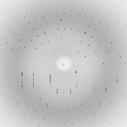
The following still image shows the result of putting a protein crystal into an X-ray beam and oscillating it back and forth by one degree around a horizontal axis. If you click on it, you will download an animated GIF file (2.8Mb) that will show how this diffraction pattern changes as we continue to rotate the crystal in one degree steps for a total of twenty degrees. Notice the lunes that move up the image, becoming a set of concentric circles for a moment.

Quantum mechanics and diffraction

As mentioned above, we can get a perfectly useful picture of diffraction by thinking in the classical terms of waves. But it may worry you that diffraction occurs one photon at a time. Very loosely, what happens in the quantum mechanical point of view is that the photon "feels" the environment of the crystal, and it randomly chooses a path with a probability determined by the wave picture we have been considering. The probability that the photon will be scattered in any particular direction is given by the square of the amplitude of the sum of the scattered waves, which we should now consider as the quantum mechanical wave function. This is why, when we measure the intensity of a diffraction spot (which is proportional to the number of photons in that spot), we take the square root as part of determining the amplitude for our electron density calculations.

Other resources

Books

T.L. Blundell & L.N. Johnson (1976), "Protein Crystallography", Academic Press: London.

Jan Drenth (1994), "Principles of Protein X-ray Crystallography", Springer-Verlag: New York.

D. Sherwood (1976), "Crystals, X-rays and Proteins", Longman: London.

Link

Bernhard Rupp's Interactive Crystallography Course.

© 1999-2009 Randy J Read, University of Cambridge. All rights reserved.

Last updated: 7 April, 2009